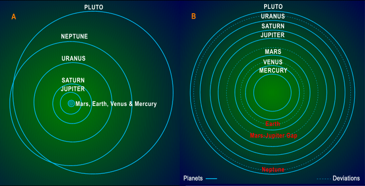
![]() Thus from a preliminary
viewpoint there are essentially four distinct regions--the first
occupied by the relatively small Terrestrial Planets, the second by the
Asteriod Belt, the third by the four immense Gas Giants and lastly the
remote and singular domain of tiny Pluto. Here one can at least begin to
regroup the data, for it is questionable whether Pluto is necessarily a
planet at all, even though it may be occupying a planetary "position"
per
se . But what constitutes a planetary position in this context anyway,
given that we have no established planetary framework to guide us? About
all that can be suggested at this stage is that Pluto, though still part
of the planetary set represents an anomaly that may or may not be explained
by further investigation. Next, a second anomaly of a different kind would
seem to be the Asteriod Belt, but while there are over 5,000 asteriods
in the region and others beyond it, their combined masses are nevertheless
far too small to account for a planet per se. But was there ever
a planet between Mars and Jupiter? Again, we simply do not know; but then
neither do we know what caused so many asteroids to be in this particular
region in the first place, though various hypothetical scenarios involving
collisions and/or the gravitational break-up of planets have been proposed
(notably by Tom Van Flandern;1 see
also the latter's Exploded
Planet Hypothesis - 2000). But here matters increase in complexity,
for orbital shifts and the redistribution of planetary masses necessarily
affect the total angular momentum of the Solar System, rotational component
of the Sun included. Which brings us to a third anomaly, namely that although
the Sun has by far the greatest mass, it is the planets--predominately
the Four Gas Giants--that possess almost all of the angular momentum. Thus
postulating orbital changes and/or the break-up of hypothetical planets
between Mars and Jupiter (or indeed anywhere in the System) involves mathematics
of N-body proportions and complexity. Difficult enough for a single occurrence,
what then of other events that may or may may not have been sequential,
periodic, or alternatively, totally unrelated in both time and place? As
for the early historical side of the matter, there are also problems and
unanswered questions that pertain to the precedence of planetary formation
itself, i.e., to what extent the Gas Giants may have preceded the Terrestrial
planets, and whether the Asteriod Belt and/or the orbit of Pluto preceded
or followed the formation of the Terrestrial Planets in turn, etc. Here
once again the matter of origins comes to the fore, as does the possibility
of catastrophic events and relatively large-scale changes within the Solar
System itself. All of which suggest that the first and foremost requirement
is an underlying planetary structure--not necessarily complete in its entirety
either, but useful enough to provide a valid starting point and an initial
frame of reference for further analysis.
Thus from a preliminary
viewpoint there are essentially four distinct regions--the first
occupied by the relatively small Terrestrial Planets, the second by the
Asteriod Belt, the third by the four immense Gas Giants and lastly the
remote and singular domain of tiny Pluto. Here one can at least begin to
regroup the data, for it is questionable whether Pluto is necessarily a
planet at all, even though it may be occupying a planetary "position"
per
se . But what constitutes a planetary position in this context anyway,
given that we have no established planetary framework to guide us? About
all that can be suggested at this stage is that Pluto, though still part
of the planetary set represents an anomaly that may or may not be explained
by further investigation. Next, a second anomaly of a different kind would
seem to be the Asteriod Belt, but while there are over 5,000 asteriods
in the region and others beyond it, their combined masses are nevertheless
far too small to account for a planet per se. But was there ever
a planet between Mars and Jupiter? Again, we simply do not know; but then
neither do we know what caused so many asteroids to be in this particular
region in the first place, though various hypothetical scenarios involving
collisions and/or the gravitational break-up of planets have been proposed
(notably by Tom Van Flandern;1 see
also the latter's Exploded
Planet Hypothesis - 2000). But here matters increase in complexity,
for orbital shifts and the redistribution of planetary masses necessarily
affect the total angular momentum of the Solar System, rotational component
of the Sun included. Which brings us to a third anomaly, namely that although
the Sun has by far the greatest mass, it is the planets--predominately
the Four Gas Giants--that possess almost all of the angular momentum. Thus
postulating orbital changes and/or the break-up of hypothetical planets
between Mars and Jupiter (or indeed anywhere in the System) involves mathematics
of N-body proportions and complexity. Difficult enough for a single occurrence,
what then of other events that may or may may not have been sequential,
periodic, or alternatively, totally unrelated in both time and place? As
for the early historical side of the matter, there are also problems and
unanswered questions that pertain to the precedence of planetary formation
itself, i.e., to what extent the Gas Giants may have preceded the Terrestrial
planets, and whether the Asteriod Belt and/or the orbit of Pluto preceded
or followed the formation of the Terrestrial Planets in turn, etc. Here
once again the matter of origins comes to the fore, as does the possibility
of catastrophic events and relatively large-scale changes within the Solar
System itself. All of which suggest that the first and foremost requirement
is an underlying planetary structure--not necessarily complete in its entirety
either, but useful enough to provide a valid starting point and an initial
frame of reference for further analysis.
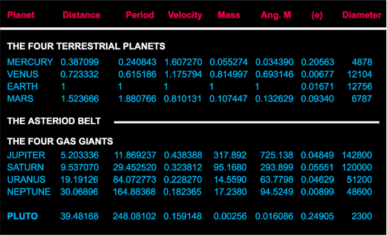
Table 1. The Nine Solar System Planets
1. Planetary masses include satellites and atmospheres.
2. Mean Heliocentric Distances in Astronomical Units (A.U).
3. Mean Periods of Revolution in Years (Harmonic Law: ref. unity).
4. Planetary diameters in kilometers.
5. (e) Eccentricities.
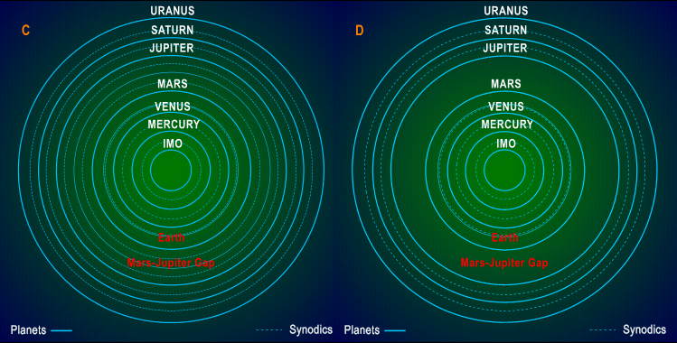
B. THE INTER-MERCURIAL OBJECT (IMO)
Additional data, i.e., physical composition, orientation of planetary
axes and planes of revolution, densities and gravities, etc., could also
have been included in Table 1, but they remain difficult to separate from
the early formation of the planetary structure itself, with or without
subsequent modifications. More in keeping with the present approach and
the need to enlarge the available database we may begin on the other hand
by adding to the nine attested planets an Inter-Mercurial Object
(called hereafter IMO) that owes its origins to orbital parameters determined
by Leverrier. Reported in the journal Nature 4
in 1876, the object in question (mean period: 33.0225 days, corresponding
mean distance 0.201438 A.U.) lies between Mercury and the Sun as the title
implies. Thus for present purposes the object serves to extend the range
of planetary mean distances at the innermost extremity, which is not to
suggest that the object is/was necessarily a planet per se, but
rather (subject to reservations already stated above) an object that may
or may not be occupying a planetary location. This step is in fact a minor
addition that although helpful is not vital to the development of the final
framework or the enlarged database; in fact the latter results largely
from the inclusion of mean periods and mean velocities in critical contexts
that will be discussed in detail later. However, before moving on to this
stage further groundwork remains; specifically the reevaulation of the
manner in which planetary orbits and parameters are generally represented.
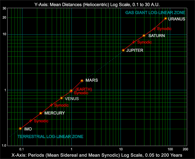
![]() Although the preliminary possibilities
suggested by the log-linear representation of the Solar System are little
more than that at present, the latter approach nevertheless provides further
avenues for investigation. In particular, the mean distances can now be
reexamined in terms of the Solar System planet-to-planet increments discussed
in Part I, but from a narrower viewpoint with a correspondingly sharper
focus. Thus the planet-to-planet multiplication factors shown below concentrate
primarily on the two indicated log-linear zones while the distances and
attendant multiplication factors for Earth and Neptune are for the time
being excluded.
Although the preliminary possibilities
suggested by the log-linear representation of the Solar System are little
more than that at present, the latter approach nevertheless provides further
avenues for investigation. In particular, the mean distances can now be
reexamined in terms of the Solar System planet-to-planet increments discussed
in Part I, but from a narrower viewpoint with a correspondingly sharper
focus. Thus the planet-to-planet multiplication factors shown below concentrate
primarily on the two indicated log-linear zones while the distances and
attendant multiplication factors for Earth and Neptune are for the time
being excluded.
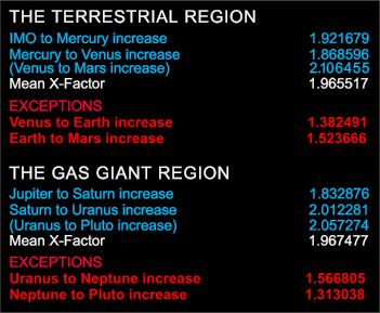
Table 2. X-Factors: Planet-to-Planet Mean Distances
The inclusion of IMO in the Terrestrial Region, the corresponding multiplication factor 1.921679 and the Venus to Mars x-factor leads to a mean value multiplier for the orbits of IMO, Mercury, Venus and Mars of 1.965517. In a similar way, the inclusion of the Uranus to Pluto x-factor results in a mean value multiplier of 1.967477 for the three adjacent planets of interest in the Gas Giant Zone (Jupiter, Saturn and Uranus). Thus the exclusion of the x-factors for Neptune and Earth results in mean multipliers in the Terrestrial and Gas Giant zones that differ by less than 0.1 percent. In other words, the mean distances in these two zones apparently increase by a multiplication factor of around 1.966... Which brings us back to Bode's Law and the suggestion of doubling for the mean distances and also, what was stated earlier, i.e., that the exponential component inherent in the latter might well have been pursued with greater forethought and vigour. But is there a constant value by which the planetary mean distance increase? In terms of the exponential framework at least, the answer is yes, but it is not something as simple as the integer 2, nor can it be determined from the information considered so far. It is in fact a precise value, i.e. 1.899547627.. obtainable to whatever degree of accuracy is desired, as will be shown in later sections.
![]() Continuing with the preliminary
indications provided by Figure 2b and as suggested in Part I, the planet-to-planet
increases for Earth and Mars may both be atypical, with Earth possibly
occupying an "intermediate" position between Mars and Venus. In Part I
it was not possible discuss the matter in further detail, but here in Table
2 the mean values provide further frames of reference, or more properly,
indexes of the proximity of adjacent planets and a tentative reference
frame for the mean distances. In other words, values that are
greater
than the mean may serve to indicate that the body in question is further
out from the Sun than the "theoretical" norm (i.e., the position corresponding
to the log-linear framework), while values that are lower are correspondingly
nearer
the Sun, etc. Thus in practice, Venus may be considered to be slightly
closer to the Sun, while Mars (because of the Venus-Mars and Earth-Mars
increases) considerably further out. Similarly, both Uranus and Pluto may
also be considered to be beyond the "norm", while Neptune--already suspected
of occupying an "intermediate" position--may be much closer in. Moreover,
the data in Table 2 also shows that the increases for the two exceptions
(Earth and Neptune) are not only similar in value, they also appear to
be reversed. Here, of course, matters are complicated by the possibility
(if not the fact) that the distances for the neighbouring planets (i.e.,
Mars in the inner zone and Uranus in the outer) may also deviate somewhat
from the "norm" for whatever cause and whatever reason. About all that
can be said at present is that these preliminary indications remain simply
that. What is required next is the introduction of synodic motion and orbital
velocity, after which the suspected deviations and anomalous locations
of Earth, Neptune and the Mars-Jupiter Gap may be revisited and examined
in further detail.
Continuing with the preliminary
indications provided by Figure 2b and as suggested in Part I, the planet-to-planet
increases for Earth and Mars may both be atypical, with Earth possibly
occupying an "intermediate" position between Mars and Venus. In Part I
it was not possible discuss the matter in further detail, but here in Table
2 the mean values provide further frames of reference, or more properly,
indexes of the proximity of adjacent planets and a tentative reference
frame for the mean distances. In other words, values that are
greater
than the mean may serve to indicate that the body in question is further
out from the Sun than the "theoretical" norm (i.e., the position corresponding
to the log-linear framework), while values that are lower are correspondingly
nearer
the Sun, etc. Thus in practice, Venus may be considered to be slightly
closer to the Sun, while Mars (because of the Venus-Mars and Earth-Mars
increases) considerably further out. Similarly, both Uranus and Pluto may
also be considered to be beyond the "norm", while Neptune--already suspected
of occupying an "intermediate" position--may be much closer in. Moreover,
the data in Table 2 also shows that the increases for the two exceptions
(Earth and Neptune) are not only similar in value, they also appear to
be reversed. Here, of course, matters are complicated by the possibility
(if not the fact) that the distances for the neighbouring planets (i.e.,
Mars in the inner zone and Uranus in the outer) may also deviate somewhat
from the "norm" for whatever cause and whatever reason. About all that
can be said at present is that these preliminary indications remain simply
that. What is required next is the introduction of synodic motion and orbital
velocity, after which the suspected deviations and anomalous locations
of Earth, Neptune and the Mars-Jupiter Gap may be revisited and examined
in further detail.
D. SYNODIC MOTION
D1-1 SYNODIC FORMULAS
![]() Although the majority of attempts
to come to terms with the structure of the Solar System have naturally
and traditionally concentrated on mean heliocentric distances, it seems
likely--especially in view of the limited amount of progress to date--that
more tools and more data are required. Given the known relationship between
mean distances and mean periods inherent in the third law of planetary
motion (see relations 2g, 2t and 2r below)--it therefore seems reasonable
to include the mean periods of revolution, though this step requires
a further expansion before it becomes usable in the present context.
Although the majority of attempts
to come to terms with the structure of the Solar System have naturally
and traditionally concentrated on mean heliocentric distances, it seems
likely--especially in view of the limited amount of progress to date--that
more tools and more data are required. Given the known relationship between
mean distances and mean periods inherent in the third law of planetary
motion (see relations 2g, 2t and 2r below)--it therefore seems reasonable
to include the mean periods of revolution, though this step requires
a further expansion before it becomes usable in the present context.
What is required is something that binds the planets together,
and for this purpose synodic periods and planetary velocities now enter into
the discussion, i.e., if the planets are indeed ordered, then the manner
in which they move with respect to each other should also be ordered,
and any ordering that involves the distances necessarily also involves both
the periods and the velocities. Which means, because of the exponential relationships
that exist between all three, that the two latter sets of parameters are also
available for present purposes.
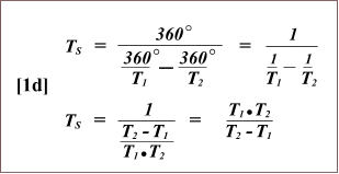
![]() In more detail, although rarely
described in the following form, for any pair of co-orbital bodies (where
T2 denotes the sidereal period of an outer body, T1 the period of revolution of an inner body, and T2 > T1) the general synodic
period (or "lap" time) may be expressed as the product of the two sidereal periods (T1
and T2) divided by their difference:
In more detail, although rarely
described in the following form, for any pair of co-orbital bodies (where
T2 denotes the sidereal period of an outer body, T1 the period of revolution of an inner body, and T2 > T1) the general synodic
period (or "lap" time) may be expressed as the product of the two sidereal periods (T1
and T2) divided by their difference:
Rel. 1a: The General Synodic Formula
Here the mean parameters of Earth provide the standard frame of reference (unity). The synodic periods of the planets are more commonly given with respect to the relative motion of Earth using simpler formulas. The latter variants are, however, merely special cases of Relation 1a with unity (the sidereal period of Earth) replacing T1 or T2 according to which group of planets is under consideration. Relation 1a is also further simplified by implicit multiplication (i.e., by unity: 1 x T2 = T2, etc.) such that:
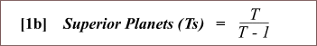
Rel. 1b: Synodic Periods ( Superior Planets )
and:
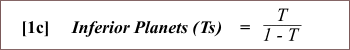
Rel. 1c: Synodic Periods ( Inferior Planets )
In view of what follows next, however, a more detailed explanation appears
to be in order. Firstly, such computations concern the time
required for a swifter co-orbital body to lap a slower orbital body, or more precisely,
the time required for one orbital body to complete 360 degrees of sidereal
motion with respect to the other.
For example, applying convenient approximate sidereal periods of revolution for Saturn and Uranus of T1 = 30 years and T2 =
90 years, the mean motion per unit time (i.e., per year)
is 360/30 = 12 degrees and 360/90 = 4 degrees respectively, resulting in an
annual difference of 8 degrees. The synodic (or lap) time of the faster planet Saturn (T1) with respect to the slower planet (Uranus, T2)
is therefore 360 degrees divided by the last result, i.e., 360/8 = 45 years. Thus the synodic period expressed in years
is obtained from the following procedure:
Rel. 1d: The Derivation of the General Synodic Formula
to arrive back at the general synodic formula (Relation 1a) and the framework for both special cases (Relation 1b and 1c).
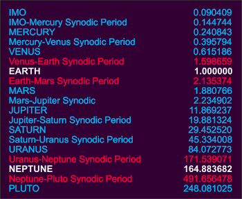
Table 3. Solar System Sidereal and Synodic Periods
Before proceeding with the next stage is seems necessary to emphasize that although the mean synodic periods represent difference or lap cycles between successive pairs of adjacent co-orbital planets, such cycles nevertheless represent complete revolutions of 360 degrees per mean synodic period. The difference between this type of orbital motion and planetary revolutions per se is that the latter take place with respect to a fixed sidereal reference point, whereas the former take place with respect to a moving point of reference. Even so, for every such mean synodic period the concept of an equivalent sidereal period and equivalent synodic "orbit" can be applied. With this device applied consistantly throughout, the equivalent synodic orbits may then be included in log-scale representations of the Solar System. Here the results serve to emphasize the log-linear aspect far more effectively than the numeric representation provided in Table 2. In fact, omitting both Neptune and Pluto for the time being, the suggestion of log-linearity appears to be quite pronounced whether planet-to-planet, synodic-to synodic, or indeed sequentially (i.e. planet-synodic-planet) in the two log-linear zones under consideration (see Figures 2c, 2d and 2e). Although no planet can be assigned to the Asteriod Belt per se, an orbit that corresponds to the geometric mean between Mars and Jupiter ( 2.8156896 A.U., sidereal period: 4.7247945 years) also provides bracketing synodic periods similar to those of the Terrestrial and Gas Giant zones, if not the continuation from the latter to the former. Not included in the table but shown in Figures 2c and 2d is the Venus-Mars synodic of 0.914222 years that lies just inside to the mean orbit of Earth. Omitted for clarity from the Figures 2c and 2d are the Earth-Mars and Mars-Jupiter synodics that with mean periods of 2.135375 years and 2.234902 years respectively lie just beyond the orbit of Mars.
SAGREDO. Allow me, please, to interrupt in order that I may point out the beautiful agreement between this thought of the Author and the views of Plato concerning the origin of the various uniform speeds with which the heavenly bodies revolve. The latter chanced upon the idea that a body could not pass from rest to any given speed and maintain it uniformly except by passing through all the degrees of speed intermediate between the given speed and rest. Plato thought that God, after having created the heavenly bodies, assigned them the proper and uniform speeds with which they were forever to revolve; and that He made them start from rest and move over definite distances under a natural and rectilinear acceleration such as governs the motion of terrestrial bodies. He added that once these bodies had gained their proper and permanent speed, their rectilinear motion was converted into a circular one, the only motion capable its desired goal.Galileo's obscure treatment of this topic is readily explained by the fact that the Dialogues Concerning Two New Sciences was written after his trial for heresy for espousing the heliocentric concept in two earlier works. Following his conviction by the Inquisition in 1633 Galileo was subsequently forced to recant and thereafter forbidden to discuss the heliocentric hypothesis again, or suffer the penalties of relapse.
···· This conception is truly worthy of Plato; and it is all the more highly prized since its undying principles remained hidden until discovered by our Author who removed from them the mask and poetical dress and set forth the idea in correct historical perspective. In view of the fact that astronomical science furnishes us such complete information concerning the size of the planetary orbits, the distances of these bodies from their centers of revolution, and their velocities, I cannot help thinking that our Author (to whom this idea of Plato was not unknown) had some curiosity to discover whether or not a definite "sublimity" might be assigned to each planet, such that, if it were to start from rest at this particular height and to fall with naturally accelerated motion along a straight line, and were later to change the speed thus acquired into uniform motion, the size of the orbit and its period of revolution would be those actually observed.SALVIATI. I think I remember his having told me that he once made the computation and found a satisfactory correspondence with the observation. But he did not wish to speak of it, lest in view of the odium which his many new discoveries had already brought upon him, this might be adding fuel to the fire. But if anyone desires such information he can obtain it for himself from the theory set forth in the present treatment. (Fourth Day [282-283], Dialogues Concerning The New Sciences, Galilei Galileo; translated by Henry Crew and Antonio de Salvio, Dover, New York 1954:259-260; emphasis supplied)

Relations 2g, 2t and 2r: The Third or Harmonic Law
to include the mean orbital velocities as follows: 5
Relations 2a-2c: Velocity Expansions of the Harmonic Law
F. INVERSE VELOCITY RELATIONSHIPS
![]() During the preliminary phase
of the present investigation, relations [2b] and [2c] were
instrumental in bringing to light that fact there presently exist in the
Solar System a pair of unusual of inverse-velocity relationships that connect
the two suspected log-linear zones. This was discovered quite accidently
during the routine preparation of mean planetary data using standard spreadsheet
techniques. As most spreadsheet users are aware, the supreme addressibility
of spreadsheets permits the "rolling" (i.e., copying) of instructions that
refer to the contents of other cells and/or columns. To produce tables
of mean planetary distances, periods and velocities, etc., it is therefore
only necessary to use one set of data (e.g., mean distances) to determine
all the rest by applying relations [1] through [2c] to adjacent columns
in the spreadsheet. It was in fact during this routine task that the Mercury-Venus-Uranus
relationship came to light during the generation of the synodic periods
when (among other things) the cell addresses and the formulas for the inverse
velocities were inadvertently applied instead of the sidereal periods.
But as happens now and again, such errors sometimes lead to potentially
more useful results than the original task itself. As for the adage: "Chance
Favours the Prepared Mind," well that too in some respects, for by this
time the investigation had been reduced to the two log-linear zones from
Mercury to Uranus with the velocity of the latter the last entry in the
column adjacent to the one containing the error. But whether accident,
"sleepwalking" in Arthur Koestler's complex sense of the term, or whatever,
this incidental relationship nevertheless provided a difference in velocities
of only 0.02 percent, i.e.,
During the preliminary phase
of the present investigation, relations [2b] and [2c] were
instrumental in bringing to light that fact there presently exist in the
Solar System a pair of unusual of inverse-velocity relationships that connect
the two suspected log-linear zones. This was discovered quite accidently
during the routine preparation of mean planetary data using standard spreadsheet
techniques. As most spreadsheet users are aware, the supreme addressibility
of spreadsheets permits the "rolling" (i.e., copying) of instructions that
refer to the contents of other cells and/or columns. To produce tables
of mean planetary distances, periods and velocities, etc., it is therefore
only necessary to use one set of data (e.g., mean distances) to determine
all the rest by applying relations [1] through [2c] to adjacent columns
in the spreadsheet. It was in fact during this routine task that the Mercury-Venus-Uranus
relationship came to light during the generation of the synodic periods
when (among other things) the cell addresses and the formulas for the inverse
velocities were inadvertently applied instead of the sidereal periods.
But as happens now and again, such errors sometimes lead to potentially
more useful results than the original task itself. As for the adage: "Chance
Favours the Prepared Mind," well that too in some respects, for by this
time the investigation had been reduced to the two log-linear zones from
Mercury to Uranus with the velocity of the latter the last entry in the
column adjacent to the one containing the error. But whether accident,
"sleepwalking" in Arthur Koestler's complex sense of the term, or whatever,
this incidental relationship nevertheless provided a difference in velocities
of only 0.02 percent, i.e.,
Relations 3a - 3b: Venus-Mercury: Uranus mean velocities
Relations 4a - 4b: Saturn-Jupiter: Mars mean velocities
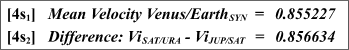
Relations 4c - 4d: Saturn/Uranus, Jupiter/Saturn: Venus/Earth mean velocites
In other words:
Vi Venus - Vi Mercury approximates the mean velocity of the planet Uranus
Vi Saturn - ViJupiter approximates the mean velocity of the planet Mars.
Vi Saturn/Uranus Synodic - ViJupiter/Saturn Synodic approximates the mean velocity of the Venus-Earth synodic cycle.
The inclusion of Earth in this context--synodic location notwithstanding--thus serves to augment the linkage between the Terrestrial planets of the lower log-linear zone and the three gas giants of the outer zone, i.e., Jupiter, Saturn and Uranus as shown in Table 4.

Table 4. The Inverse Velocity Relationships, Synodics, and the Two Log-Linear Zones
One or two other inverse-velocity relationship also appear to exist that are almost sequential--a qualifier necessary here in so much as the latter appear to incorporate synodics and planetary inverse velocities. But there are also other considerations and complications to be addressed, for although mean values are applied in these relationships, in real time such functions vary according to the elliptical natures of the associated orbits. Nevertheless, in the case of the Mars-Jupiter-Saturn relationship, with frames of reference provided by the mean orbital velocity of Earth of 29.7859 kilometers per second and 24.1309 kilometers per second for that of Mars, real-time maxima and minima for Relation [4b] range between 19.66 and 28.3 kilometers per second, thus well exceeding the extremal velocities of Mars itself. However, utilizing the methods of Bretagon and Simon7 adapted to generate sequential data for 5-day intervals from 1700 to 2000 A. D., the mean value nevertheless still turns out to be 24.0938 kilometers per second, as shown in Figure 2e below for the interval 1900 to 2000 (velocities relative to unity).
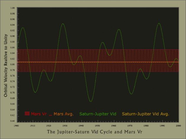
Figure 2e. The 60-Year Saturn-Jupiter Vid (Inverse velocity) cycle: 1900 - 2000
Similarly, the data for the real-time function based on Relation [4s1] reveals that although there is an even wider swing in extremal values, the mean value is also comparable to that obtained from Relation [4s1] directly. All of which is further complicated by the proximity of the Mars-Jupiter synodic to the Earth-Mars synodic and various resonances known to exist in the Solar System--complications that at this stage no doubt intrude rather than enlighten and as such will be deferred for the time being.
Finally, suffice it to note here that although only a few inverse-velocity
relationships are readily apparent in the Solar System and the scarcity
might suggest these relations have little to do with the log-linear sequences,
it turns out that they are in fact an integral feature with corresponding
values for all planetary and synodic positions. The reason for there being
so few would appear to lie in the fact that the inverse-velocity relationships
are influenced in no small way by deviations in the planetary structure.
Thus with three suspected deviations to contend with it is perhaps fortunate
that those that were evident were sufficient to connect the two
log-linear zones in the manner discussed above.
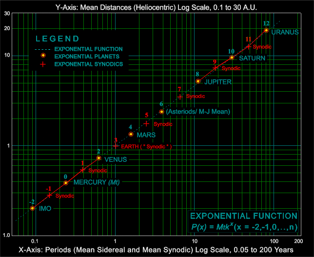
![]() To summarize the investigation
so far, there are indications that in spite of a number of anomalies, the
Solar System may possess two log-linear zones separated by the Asteriod
Belt. With the addition of the intervening synodic periods and the inverse-velocity
relationships, it can be tentatively suggested that there are essentially
five consecutive inter-related periods in the outer zone, and (with IMO
included) five more in the inner zone, or with the further inclusion of
Mars, seven as emphasized below in Figure 2f.
To summarize the investigation
so far, there are indications that in spite of a number of anomalies, the
Solar System may possess two log-linear zones separated by the Asteriod
Belt. With the addition of the intervening synodic periods and the inverse-velocity
relationships, it can be tentatively suggested that there are essentially
five consecutive inter-related periods in the outer zone, and (with IMO
included) five more in the inner zone, or with the further inclusion of
Mars, seven as emphasized below in Figure 2f.
the first expansion Mk1 is directly obtainable
from the product of the mean sidereal periods of Mercury and Venus
divided by their difference:
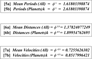
lead in turn to the determination that the value of k for the fundamental periods of the Solar System is constant Phi = 1.6180339887949, the "Golden Section" known and revered since antiquity, defined in turn by the resulting quadratic equation (Livio, 2002) 8
Relations 5a-7b. Primary Pheidian Constants: Periods, Distances and Velocities
At which, point, now that we
have arrived at the required constant of linearity and found it to be the Golden Section,
two prime related sources may be supplied:
1. The Fibonacci Numbers and the Golden section Site ( http://www.mcs.surrey.ac.uk/Personal/R.Knott/Fibonacci/fib.html )
2. The Museum of Harmony and the Golden Section ( http://www.goldenmuseum.com/index_engl.html ).
In particular with respect to the above determination, from the latter: The Geometrical Definition of the Golden Section and also Music of the Celestial Orbits with its reference to the researches of Russian astronomer K. P. Butusov, who in 1978:9
"established, that the ratios of the adjacent planets cycle times around of the Sun are equal to the golden proportion 1.618, or its square 2.618. "
which is, of course, essentially the above result.
Dr. K. P. Butusov also provides (among other determinations) related Planetary Period and Planetary Distance Laws in the following abstract:
Butusov K.P.
In the work it is demonstrated, that in a field of acoustic waves, that are aroused at the account of the tidal action of planets, there may exist a special resonance, which we have called « beating waves resonance ». This resonance arises wherever there exists equality between beating period and the sum or difference of the circulation periods of the two neighbouring planets (Beating period - being a quantity inverse of the difference between planets circulation frequences). In case of the sum, the periods ratio is equal to θ - the Phidias Number, (θ = 1.6180339), while in case of the difference the periods ratio is equal to θ2, (θ2 = 2.6180339). On this basis law was formulated named a Planet Periods Law, which says, that planets circulation periods form number sequences of Fibonacci and the one of Lucas. In second case the orbit radii form a geometrical progression with denominator θ4/3 (θ4/3 =1.899546). According to the Planet Distances Law of Johannes Titius, the orbit radii form a geometrical progression with the denominator 2, even though observational data give a value of 1.9. So we think that the Planet Distances Law - is a sequel of the beating waves resonance and, accordingly, of the Planet Periods Law. ( http//www.shaping.ru/mku/butusovart/05/05.pdf )
Thus the initial lines of inquiry may be different, but the same exponential framework and fundamental constants nevertheless result.
Return to Spira Solaris
Previous Section
Next
Section