
A. CHAOTIC SYNODIC CYCLES
THE FOUR MAJOR SUPERIOR PLANETS
The methodology provided by Betagnon and Simon in:
TABLES FOR THE MOTION OF THE SUN AND THE FIVE PLANETS FROM - 4000 TO + 2800
TABLES FOR THE MOTION OF URANUS AND NEPTUNE FROM + 1600 TO + 2800
Pierre Bretagnon and Jean-louis Simon
Service des Calculs et de Mé
77, avenue Denfert-Rochereau, 75014 Paris, France. Published by Willmann-Bell, Inc., Richmond, 1986.
initially determines the heliocentric
radius vectors, heliocentric longitudes and the heliocentric latitudes
for specific dates for the four major superior planets.
Although originally utilising BASIC and intended for single events, the
method may be adapted to other programming languages and
expanded to provide sequential heliocentric data sufficient enough to generate plan-view
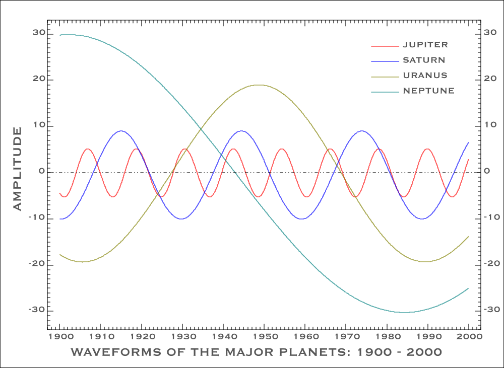
orbits and sinusoidal plots of real-time planetary motion, etc. For example,
the waveforms and phase relationships for the major planets are shown below
for the period 1900-2000 AD generated in 5-day increments with 7,300
data points for each planet:

Larger (1000 x 730)
SINGLE AND COMPOUND SYNODIC CYCLES
A real-time synodic function that describes the motions of adjacent planets
depends on the determination of the respective radius vectors, the corresponding
velocities and the corresponding periods of the two planets in question.
In dealing with the relative motions of planets in this manner, however,
it becomes feasible to undertake investigations that were hitherto numerically
impractical. One might, for example combine adjacent synodic cycles, i.e.,
for four adjacent planets the first and second synodic cycles may
be combined to form a further synodic with the same technique applied to
the third and fourth synodics and so on until one single synodic difference
function is obtained. All that is required to accomplish this goal are
simultaneous values for the radius vectors of the planets in question.
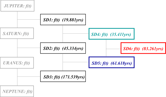
For the four adjacent superior planets Jupiter, Saturn, Uranus and Neptune
this requirement is readily met by the power series data and formulas provided
by Bretagnon and Simon (1986) outlined in the
previous section.
In other words, with values known for the radius vectors for the four
major superior planets
at any specified point in time, theoretical orbital "periods" are
also available, i.e., for each radius vector R(t) there exists a
theoretical mean orbital period of revolution P(t), and
corresponding orbital velocity, V(t) -- both readily obtained from
Kepler's Third Law in full: P 2 = R 3 = V -6.
Next, with the corresponding Periods determined in this way, the
orbital motions of the four major superior planets may be reduced to
one single variable function SD6 (t) by applying the general synodic formula:
such that Synodic Difference cycle 1 (SD1 ) is determined from the
relative motion of Jupiter with respect to Saturn, SD2 from
the relative motion of Saturn with respect to Uranus, and SD3
from the relative motion of Uranus with respect to Neptune. By treating SD1, SD2 and SD3 as equivalent "orbital" periods, the same process may then be repeated, thus synodic difference cycle SD4 is produced from SD1
and SD2, and in a similar mannner, SD5 obtained from SD2
and SD3. The new pair (SD4 and SD5) finally produce, in like manner SD6, thus a single function derived from the instantaneous
relative motions of all four planets.
The mean values (in
years) for the six cycles are as follows:
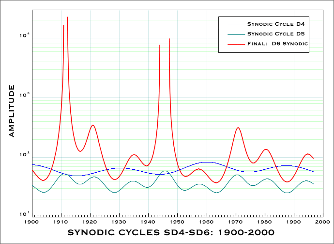
As it turns out, for both the mean periods and the real time variations,
synodic difference cycles
SD1 through
SD5 are
all well-behaved functions that swing between the limits imposed by the
elliptical orbits of the planets in question. However, although the two
synodic difference cycles that determine
SD6 are both stable,
there are points in time when the periods of the final pair
(SD4
and
SD5 ) intersect and crossover (see below) which causes
SD6
to become chaotic. The interaction between the three final synodic cycles
over the interval
1900-2000 ( 5-day increments and 7,300 data points
) shows that in the present century there were two main chaotic phases
that commenced in
1911 and
1943 respectively..
SD6 AND SOLAR ACTIVITY CYCLES
The fact that there is a chaotic component associated with the combined
motions of the four major superior planets is of some interest, especially
when it is remembered that these four adjacent bodies together possess
more than 97 percent of the angular momentum in the Solar System
as well as most of the orbital mass. In fact further examination of SD6
reveals the existence of an approximate 178-year cycle that suggests
the function may have some connection with the solar activity cycle, given
that a 178-year interval and a 45-year cycle have already
been tentatively associated with solar activity. In passing it is also
relevant to note here that although it was customary in the past to consider
sunspots numbers in terms of an eleven-year cycle, the latter is nevertheless
the average value of a cycle with observed extrema that range between
8 and 13 years. Moreover, it is also now realized that sunspots return
to the same polarity after a 22-year interval - again an average
period. Whereas the mean synodic cycle between Jupiter and Saturn
is some 19.88 years and the function itself theoretically ranges
from approximately 16.8 years to 21.2 years.
Nevertheless, irrespective of whether the major planets are currently believed
to have a minimal effect on the Sun or not, these cycles (especially the
178-year interval ) are nevertheless worthy of further examination.
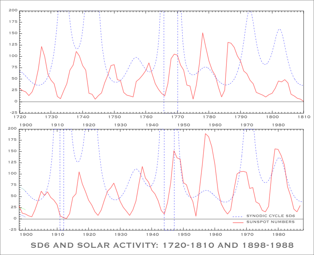
Thus in the following example the 178-cycle and SD6
are plotted against smoothed sunspot numbers from 1720 to 1820
and 1898 to1988. The times-series synodic data here are again
computed for consecutive 5-day intervals. For clarity SD6 is
truncated where the function becomes chaotic; points of particular interest
occur in 1765 and 178 years later in 1943; both are
in fact times of sunspot minima that preceded higher than normal maxima.
Further times of interest are the sunspot minima that occur around 1733
and 1911, both again chaotic points separated by an interval of
178
years. Further times-series analysis from 1600 through
2000 AD
suggests that SD6 is a complex function that may provide
additional insights although it need not be the major factor in the given
context.

Larger ( 1000 x 810 )
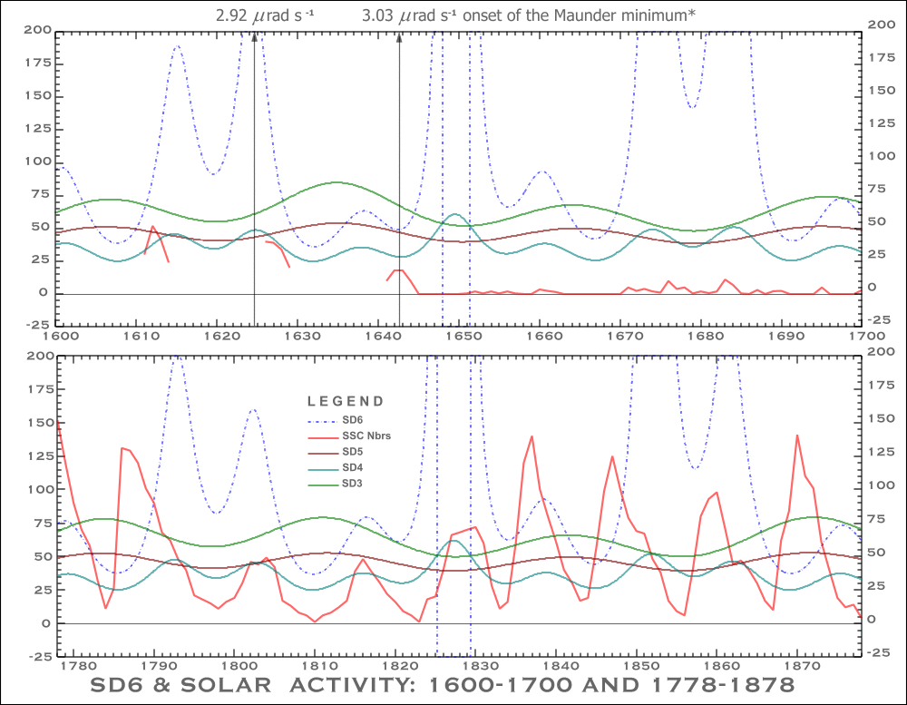
SD6, SOLAR ACTIVITY, SOLAR ROTATION RATES, AND THE MAUNDER MINIMUM
"ANOMALOUS SOLAR ROTATION IN THE EARLY 17TH CENTURY"
Eddy, John A., et al: Science, 198:824-829, 1977.
ABSTRACT
"The character of solar rotation has been examined for two periods in
the 17th century for which detailed sunspot drawings are available:
A.D. 1625 through 1626 and 1642 through 1644. The
first period occurred 20 years before the start of the Maunder sunspot
minimum, 1645 through 1715; the second occurred just at its
commencement. Solar rotation in the earlier period was much like
that of today. In the later period, the equatorial velocity of the sun
was faster by 3 to 5 percent and the differential rotation was enhanced
by a factor of 3. The equatorial acceleration with declining
solar activity is in the same sense as that found in recent doppler
data. It seems likely that the change in rotation of the solar surface
between 1625 and 1645 was associated with the onset of the Maunder
minimum."

Larger ( 1000 x 780 )
*SOLAR ROTATION RATES: 1625, 1642
Norm: 2.9 urad s -1 at the solar equator
In 1625: 2.92 urad s -1
In 1642: 3.03 urad s -1
(The Sun as a Star, Ed. Stuart Jordon, NASA, 1981:17)
B. RESONANT SYNODIC CYCLES
THE INFERIOR PLANETS
One of the main advantages of time-series analysis is the ability to investigate
complex interactions that are neither indicated nor suspected from mean
or extremal values. A case in point concerns the relationships between
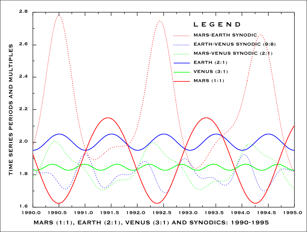
the three inferior planets Venus, Earth and Mars. Irrespective of whether
one considers that Earth presently occupies a synodic rather than
planetary position between Venus and Mars or not, the synodic cycles
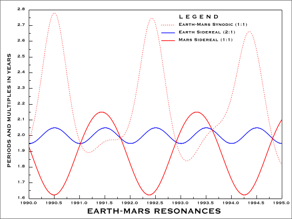
in question are undoubtedly complex. It is well known, for example, that
Earth is in 2 : 1 resonant relationship with Mars; what is
not so well understood, however, is when and where such resonances actually
take place. Here again it is a matter of computing periodic functions,
in this case the sidereal motions of the two planets in question plus the
varying synodic cycle. A plot of the resulting time series data in 1-day
increments from 1990 to 1995 (1828 data points) is shown below:
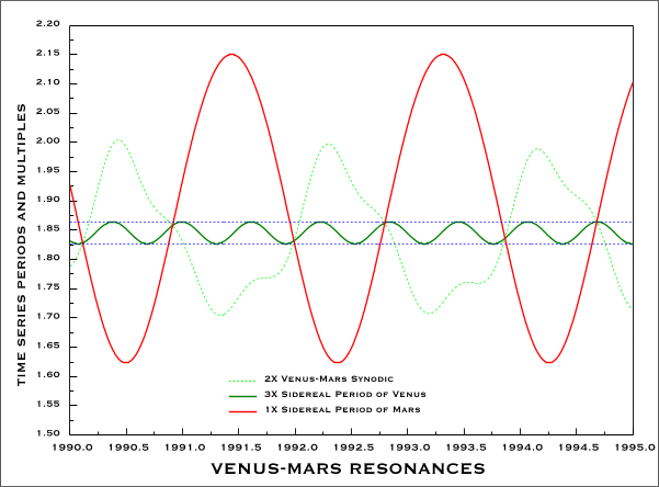
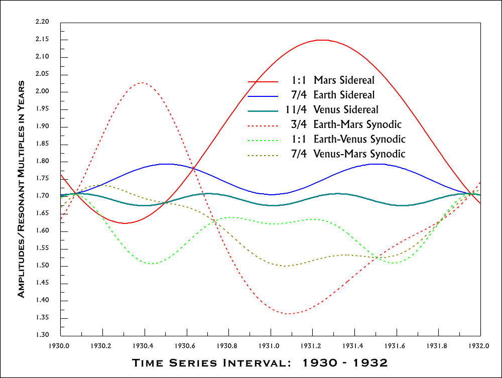
A similar approach may be adopted to include Venus. Here the investigation
can be extended to include the determination of fractional constants and
whole number multiples such that the synodic and sidereal cycles intersect.
An example of the latter is shown in the following graph:
Next, combining all three inferior planets in the same manner including integer and fractional constants we also obtain:

Larger (1000 x 760)
Lastly, a Lucas-series variant:

Larger (1000 x 750)
Time
Series Analyisis
Return to Spira Solaris
Copyright © 1998. John N. Harris, M.A.(CMNS). Last Updated on July 16, 2004