

PLANETARY MOTION, SINGLE-EVENT AND TIME SERIES FORMULAS
A. THE MAJOR SUPERIOR PLANETS
The methodology and formulas applied to planetary motion in this context
are provided by Pierre Bretagnon and Jean-Louis Simon in Planetary Programs
and Tables from - 4000 to +2800 (Willman-Bell, Richmond, 1986). The
astronomical programs in this work concern the determination of the positions
of the planets as viewed from Earth (i.e., geocentric coordinates with
corrections for aberration, nutation, and precession, etc). The first stage,
however, concerns the determination of heliocentric coordinates. For Jupiter,
Saturn, Uranus and Neptune the latter are obtained from the following power
series formulas:
HELIOCENTRIC LONGITUDE (L)
HELIOCENTRIC LATITUDE (B)

HELIOCENTRIC RADIUS VECTOR (R)

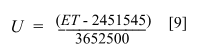
The parameter V is measured in units of 2000 julian days from the beginning of successive five-year intervals; the units are radians for L and B, and astronomical units ( AU ) for R. Tables for the motion of Jupiter, Saturn, Uranus and Neptune are obtained from power series data for five-year intervals, e.g., for the period 1990 to 1995 BP starting with Julian Day 2447892.5 the tables are as follows [Bretagnon and Simon 1986:124, 140]:
JUPITER 1990 2447892.5
L) 1.678682 2.956725 -0.414596  0.004826 0.299734 -0.151349  0.029332
B)-0.005204 0.067083 -0.000759 -0.109760 0.078191 -0.029462  0.007110
R) 5.155577 0.717884  0.187303 -1.133334 0.310164  0.141854 -0.042529
L) 4.993758 1.054503  0.014505 0.023160 -0.000553 -0.000863 -0.000059
B) 0.005629-0.045382 -0.003796 0.007466  0.000345  0.000362 -0.000177
R)10.027146-0.144092 -0.300680 0.032117  0.003847  0.022473 -0.008193
L) 4.808885 0.401780 -0.007396 0.001186 -0.000138 -0.000220  0.000115
B)-0.004951-0.000503  0.000528-0.000054  0.000306 -0.000299  0.000108
R)19.380045 0.357595 -0.005398-0.008060 -0.013812  0.011760 -0.004261
L) 4.923200 0.207762  0.000166 0.000853 -0.000671  0.000373 -0.000118
B) 0.015270-0.005562 -0.000339 0.000013  0.000032 -0.000016  0.000004
R)30.210400-0.047301  0.013832 0.001610 -0.018511  0.014834 -0.005138

where T0 is the beginning julian date of the
time-span,
T i is the required point in time for
the superior planet (s) in question and V ranges from 0 to 0.915.
REAL-TIME PLANETARY ORBITS
Plan-view plots of planetary orbits require the computation of the heliocentric
longitude (L) and the heliocentric radius vector (R)
for successive values of V within a given time-span. However,
none of the major superior planets have sidereal periods that are shorter
than five years thus the computation of each orbit entails the use of successive
five-year data sets. For one complete orbit of Jupiter, a minimum of two sets of
data is required; for Saturn five, Uranus seventeen, and for Neptune thirty-three.
For the interval 1600 - 2100 BP, one hundred consecutive
sets of power series data are therefore required for each planet.
B. THE FOUR TERRESTRIAL PLANETS
In contrast to the relatively simple power-series methodology
for the major superior planets formulas for the terrestrial planets
are both cumbersome and difficult to implement in times-series format
without
the heavy use of computing devices. Here the formulas vary from planet to planet
and all require tables and lengthy trigonometric summations. For
example, for Mercury alone the formulas and tables for the heliocentric
radius vector (R), the heliocentric latitude (B), and the heliocentric
longitude (L) are:
MERCURY: HELIOCENTRIC RADIUS VECTOR ( R )
| i | ri | ai | vi |
| 1 | 780141 | 6.202782 | 260878.753962 |
| 2 | 78942 | 2.98062 | 521757.50830 |
| 3 | 12000 | 6.0391 | 782636.264 0 |
| 4 | 9839 | 4.8422 | 260879.380 8 |
| 5 | 2355 | 5.062 | 0.734 |
| 6 | 2019 | 2.898 | 1 043514.987 |
| 7 | 1974 | 1.588 | 521758.140 |
| 8 | 1859 | 0.805 | 260877.716 |
| 9 | 426 | 4.601 | 782636.915 |
| 10 | 397 | 5.976 | 1 304393.735 |
| 11 | 382 | 3.86 | 521756.47 |
| 12 | 306 | 1.87 | 1 043515.34 |
| 13 | 102 | 0.62 | 782635.28 |
| 14 | 92 | 2.60 | 1 565272.52 |
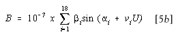
TABLE: i = 1 to 18
| i | bi | ai | vi |
| 1 | 680303 |
3.82625 |
260879.17693 |
| 2 | 538354 |
3.30009 |
260879.66625 |
| 3 | 176935 |
3.74070 |
0.40005 |
| 4 | 143323 |
0.58073 |
521757.92658 |
| 5 | 105214 |
0.05450 |
521758.44880 |
| 6 | 91011 |
3.3915 |
0.9954 |
| 7 | 47427 |
1.9266 |
260878.2610 |
| 8 | 41669 |
3.5084 |
782636.7624 |
| 9 | 19826 |
3.1539 |
782637.4813 |
| 10 | 12963 |
0.2455 |
1043515.6610 |
| 11 | 8233 |
4.886 |
521756.972 |
| 12 | 6399 |
0.358 |
782637.769 |
| 13 | 3196 |
3.253 |
1304394.380 |
| 14 | 1536 |
4.824 |
1043516.451 |
| 15 |
824 |
0.04 |
1565273.15 |
| 16 | 819 |
1.84 |
782635.45 |
| 17 | 324 |
1.60 |
1304395.53 |
| 18 | 201 |
2.92 |
1826151.86 |
L = 4.4429839 + 260881.4701279U
+10-6{(409894.2+2435U-1408U 2 +114U 3 +233U 4 -88U 5 )
x sin(3.053817+260878.756773U-0.001093U 2 +0.00093U 3+0.00043U 4+0.00014U 5)}
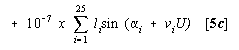
TABLE: i = 1 to 25
| i | Li | ai | vi |
| 1 | 510728 |
6.09670 |
521757.52364 |
| 2 | 404847 |
4.72189 |
1.62027 |
| 3 | 91048 |
2.8946 |
782636.2744 |
| 4 | 30594 |
4.1535 |
521758.6270 |
| 5 | 15769 |
5.8003 |
1043515.0730 |
| 6 | 13726 |
0.4656 |
521756.9570 |
| 7 | 11582 |
1.0266 |
782638.007 |
| 8 | 7633 |
3.517 |
521759.335 |
| 9 | 5247 |
0.418 |
1043516.352 |
| 10 | 4001 |
3.993 |
1304393.680 |
| 11 | 3299 |
2.791 |
1043514.724 |
| 12 | 3212 |
0.209 |
1304394.627 |
| 13 | 1690 |
2.067 |
1304395.168 |
| 14 | 1482 |
6.174 |
782635.409 |
| 15 |
1233 |
3.606 |
1043516.88 |
| 16 | 1152 |
5.856 |
1565272.646 |
| 17 | 845 |
2.63 |
1565273.50 |
| 18 | 654 |
3.40 |
1826151.56 |
| 19 | 359 |
2.66 |
11094.77 |
| 20 | 356 |
3.08 |
1565273.50 |
| 21 | 257 |
6.27 |
1826152.20 |
| 22 | 246 |
2.89 |
5.41 |
| 23 | 180 |
5.67 |
56613.61 |
| 24 | 159 |
4.57 |
250285.49 |
| 25 | 137 |
6.17 |
271973.50 |
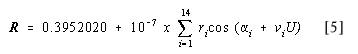
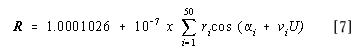
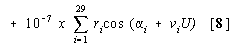
HELIOCENTRIC RADIUS VECTORS: VENUS, SUN (EARTH), AND MARS
R = 0.723 5481 + 10 -7 {(48982 - 34549U + 7096U 2 3360U 3 + 890U 4 - 210U 5)
x cos(4.02152 + 102132.84695U + 0.2420U 2 + 0.0994U 3 + 0.0351U 4 - 0.0013U 5 - 0.015U 6)}
+ 10-7{(166-234U + 131U 2) x cos(4.90 + 204265.69U + 0.48U 2 + 0.20U 3)}
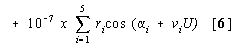
TABLE: i = 1 to 5
| i | ri | ai | vi |
| 1 | 72101 | 2.828 | 0.361 |
| 2 | 163 | 2.85 | 78604.20 |
| 3 | 138 | 1.13 | 117906.29 |
| 50 | 2.59 | 96835.94 | |
| 5 | 37 | 1.42 | 39302.10 |
[Table: i = 1 to 50 omitted ]
MARS: HELIOCENTRIC RADIUS VECTOR (R)
R = 1.5298560 + 10-6{(141 849.5 + 13651.8U - 1230U 2 - 378U 3 + 187U 4 - 153U 5 - 73U 6)
cos(3.479698+33405.349560U+0.030669U2 -0.00909U3+0.00223U4 +0.00083U5 -0.00048U6)}
+ 10-6{(6607.8 + 1272.8U - 53U 2 - 46U 3 + 14U 4 - 12U 5 + 99U 6)x
cos(3.81781 + 66810.6991U + 0.0613U 2 - 0.0182U 3 + 0.0044U 4 + 0.0012U 5 + 0.002U 6)}
TIME
TABLES FOR THE MOTION OF THE SUN AND THE FIVE PLANETS FROM - 4000 TO + 2800
TABLES FOR THE MOTION OF URANUS AND NEPTUNE FROM + 1600 TO + 2800
Pierre Bretagnon and Jean-louis Simon
Service des Calculs et de Mécanique Céleste du Bureau des Longitudes
77, avenue Denfert-Rochereau, 75014 Paris, France.
Published by Willmann-Bell, Inc., Richmond, 1986.
Return to Spira Solaris
[] Times Series Graphics